1. 滑动窗口
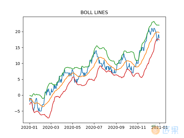
所谓时序的滑窗函数,即把滑动窗口用 freq 关键词代替,下面给出一个具体的应用案例:在股票市场中有一个指标为 BOLL 指标,它由中轨线、上轨线、下轨线这三根线构成,具体的计算方法分别是 N 日均值线、 N 日均值加两倍 N 日标准差线、 N 日均值减两倍 N 日标准差线。利用 rolling 对象计算 N=30 的 BOLL 指标可以如下写出:
In [101]: import matplotlib.pyplot as plt
In [102]: idx = pd.date_range('20200101', '20201231', freq='B')
In [103]: np.random.seed(2020)
In [104]: data = np.random.randint(-1,2,len(idx)).cumsum() # 随机游动构造模拟序列
In [105]: s = pd.Series(data,index=idx)
In [106]: s.head()
Out[106]:
2020-01-01   -1
2020-01-02   -2
2020-01-03   -1
2020-01-06   -1
2020-01-07   -2
Freq: B, dtype: int32
In [107]: r = s.rolling('30D')
In [108]: plt.plot(s)
Out[108]: [<matplotlib.lines.Line2D at 0x2647d226f48>]
In [109]: plt.title('BOLL LINES')
Out[109]: Text(0.5, 1.0, 'BOLL LINES')
In [110]: plt.plot(r.mean())
Out[110]: [<matplotlib.lines.Line2D at 0x2647d290ac8>]
In [111]: plt.plot(r.mean()+r.std()*2)
Out[111]: [<matplotlib.lines.Line2D at 0x2647d290908>]
In [112]: plt.plot(r.mean()-r.std()*2)
Out[112]: [<matplotlib.lines.Line2D at 0x2647d29b748>]
对于 shift 函数而言,作用在 datetime64 为索引的序列上时,可以指定 freq 单位进行滑动:
In [113]: s.shift(freq='50D').head()
Out[113]:
2020-02-20   -1
2020-02-21   -2
2020-02-22   -1
2020-02-25   -1
2020-02-26   -2
dtype: int32
另外, datetime64[ns] 的序列进行 diff 后就能够得到 timedelta64[ns] 的序列,这能够使用户方便地观察有序时间序列的间隔:
In [114]: my_series = pd.Series(s.index)
In [115]: my_series.head()
Out[115]:
0   2020-01-01
1   2020-01-02
2   2020-01-03
3   2020-01-06
4   2020-01-07
dtype: datetime64[ns]
In [116]: my_series.diff(1).head()
Out[116]:
0      NaT
1   1 days
2   1 days
3   3 days
4   1 days
dtype: timedelta64[ns]
2. 重采样
重采样对象 resample 和第四章中分组对象 groupby 的用法类似,前者是针对时间序列的分组计算而设计的分组对象。
例如,对上面的序列计算每10天的均值:
In [117]: s.resample('10D').mean().head()
Out[117]:
2020-01-01   -2.000000
2020-01-11   -3.166667
2020-01-21   -3.625000
2020-01-31   -4.000000
2020-02-10   -0.375000
Freq: 10D, dtype: float64
同时,如果没有内置定义的处理函数,可以通过 apply 方法自定义:
In [118]: s.resample('10D').apply(lambda x:x.max()-x.min()).head() # 极差
Out[118]:
2020-01-01    3
2020-01-11    4
2020-01-21    4
2020-01-31    2
2020-02-10    4
Freq: 10D, dtype: int32
在 resample 中要特别注意组边界值的处理情况,默认情况下起始值的计算方法是从最小值时间戳对应日期的午夜 00:00:00 开始增加 freq ,直到不超过该最小时间戳的最大时间戳,由此对应的时间戳为起始值,然后每次累加 freq 参数作为分割结点进行分组,区间情况为左闭右开。下面构造一个不均匀的例子:
In [119]: idx = pd.date_range('20200101 8:26:35', '20200101 9:31:58', freq='77s')
In [120]: data = np.random.randint(-1,2,len(idx)).cumsum()
In [121]: s = pd.Series(data,index=idx)
In [122]: s.head()
Out[122]:
2020-01-01 08:26:35   -1
2020-01-01 08:27:52   -1
2020-01-01 08:29:09   -2
2020-01-01 08:30:26   -3
2020-01-01 08:31:43   -4
Freq: 77S, dtype: int32
下面对应的第一个组起始值为 08:24:00 ,其是从当天0点增加72个 freq=7 min 得到的,如果再增加一个 freq 则超出了序列的最小时间戳 08:26:35 :
In [123]: s.resample('7min').mean().head()
Out[123]:
2020-01-01 08:24:00   -1.750000
2020-01-01 08:31:00   -2.600000
2020-01-01 08:38:00   -2.166667
2020-01-01 08:45:00    0.200000
2020-01-01 08:52:00    2.833333
Freq: 7T, dtype: float64
有时候,用户希望从序列的最小时间戳开始依次增加 freq 进行分组,此时可以指定 origin 参数为 start :
In [124]: s.resample('7min', origin='start').mean().head()
Out[124]:
2020-01-01 08:26:35   -2.333333
2020-01-01 08:33:35   -2.400000
2020-01-01 08:40:35   -1.333333
2020-01-01 08:47:35    1.200000
2020-01-01 08:54:35    3.166667
Freq: 7T, dtype: float64
在返回值中,要注意索引一般是取组的第一个时间戳,但 M, A, Q, BM, BA, BQ, W 这七个是取对应区间的最后一个时间戳:
In [125]: s = pd.Series(np.random.randint(2,size=366),
   .....:               index=pd.date_range('2020-01-01',
   .....:                                   '2020-12-31'))
   .....:
In [126]: s.resample('M').mean().head()
Out[126]:
2020-01-31    0.451613
2020-02-29    0.448276
2020-03-31    0.516129
2020-04-30    0.566667
2020-05-31    0.451613
Freq: M, dtype: float64
In [127]: s.resample('MS').mean().head() # 结果一样,但索引不同
Out[127]:
2020-01-01    0.451613
2020-02-01    0.448276
2020-03-01    0.516129
2020-04-01    0.566667
2020-05-01    0.451613
Freq: MS, dtype: float64